Methodology
A project involving carbon nanotubes (CNTs) provides an example.
Carbon nanotubes have become the basis of intense research due to their intriguing mechanical and electrical properties. In Motorola’s Embedded Research Systems Laboratory CNT’s electrical conductivity and high aspect ratio (length in the m, diameters in the nm range) have been utilized in one particular application for field emitter displays. The adjacent image shows a 4.6-inch display where millions of CNTs have been selectively deposited on a glass cathode while their emission has been regulated for display function.
Such fully processed displays represent a considerable resource commitment due to their manufacturing complexity. Therefore, blanket, non-patterned, diode samples were initiated as test and optimization vehicles. CNT growth was achieved by a two-step deposition process – first a metallic catalyst is deposited in a separate tool, followed by the deposition of the CNTs in a chemical vapor deposition reactor. After deposition of the CNTs, the emission properties were investigated by extracting the emission current on an anode and exposing the CNTs to an electric field. The current density was an indicator of brightness, convoluted by the phosphorus efficacy of the anode.
The brightness of the display was maximized using a classical design of experiments (DOE) approach in what is called subsequently the “laboratory phase.” The most efficient method for optimization is a sequential approach that is partitioned into three separate components – screening DOE, path of steepest ascent (PoA) and response surface method (RSM), as illustrated in Figure1. Off-the-shelf software was used for the statistical analysis. The sequential experimental approach allowed for resource efficient optimization of the emission current density. Typically, this three-tiered approach is now used in Monte Carlo simulation to predict the process variability followed by laboratory verification runs. In the approach illustrated in Figure 1, it is demonstrated that the Monte Carlo simulation in what is termed the “simulation phase” also can be used as a process troubleshooting tool and may lead to discoveries of hidden influential factors. Simulation software was used to carry out the Monte Carlo simulation. The statistical model obtained from the laboratory phase was used as a transfer function to calculate the expected emission output current density. Since the control of the significant factors is limited, their variation led to a distribution of the resulting emission current density.
The DOE demonstrated that the output distribution is critically dependent on the input variation distributions. By systematically changing the significant factor distribution in a computer experiment, a good fit to the measured emission current density was obtained. Then the obtained response model can be analyzed for its sensitivity to the input distributions. The response model also can be used to detect significant deviations, for example, deviations caused by a process shift, from the expected output curve.
Figure 1: Flowchart of the Experimental Procedure
Laboratory Phase
A screening DOE (½ fraction of a 2-level, 4-factor resolution, IV, 24-1IV) was carried out in the initial phase to reveal what factors had significant influence on the emission current. The Pareto chart in Figure 2 identifies the two most significant factors, A and B, whereas D had only a minor influence. It also shows that some interaction between A and B was present and Factor C had no impact. The inset displays the residuals of the statistical model plotted against the most significant Factor A. The response surface was curved; therefore a RSM was required for true optimization.
Figure 2: Pareto Chart of the Standardized Effects
Figure 3: Contour Plot of Transformed Emission Current Density
Figure 4: Contour Plot of Emission Current Density (mA/cm2)
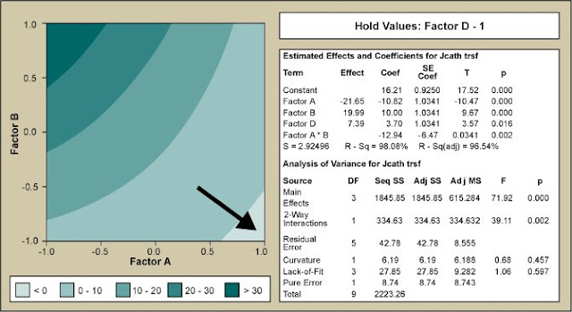
In the contour plot of Figure 3, an inverse square root transformation was used on the emission current density to normalize the data and plotted versus the two most significant factors – A and B. The analysis of variance (ANOVA) table is given in the inset. Results of Figure 3 indicated that in order to improve emission current density, Factor A should be increased and Factor B decreased. This course was pursued with the PoA. It rapidly became clear that while Factor A was easily controlled and increased, Factor B was not. Lowering Factor B below a certain threshold resulted in loss of controllability and a compromise had to be found. Therefore the most flexible and most important factor was Factor A. As Factor A was steadily increased a local maximum for emission current was found with the RSM centered on that new high point.
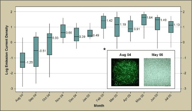
The results of the RSM are shown in Figure 4 with the ANOVA table as an inset. The contour map of the model obtained by the analysis indicates the region of maximized emission current. Figure 5 illustrates the effect of the optimization experiments. The boxplot summary of the emission current density is shown over time grouped by month. The current density is plotted on a logarithmic scale (each of the dashed lines representing one order of magnitude) and the median values for each month are indicated in bold numbers. It can easily be seen that the improvement equates to more than three orders of magnitude (from ca. -1.25 to ca. to +1.3, averaged over the last six months). The two images of the inset of Figure 5 illustrate the increase in brightness. The shutter speed of the camera had to be reduced by ca. 100x due to the much higher emission after the RSM. If the camera shutter speed had been left the same, the right image would be overexposed. Nonetheless, the improvement is not only noticeable in the brightness but also in the much higher density of emitters.
Figure 5: Box Plot of Emission Current Density Over Time
To this point the CNT growth project appeared to be a conventional Six Sigma DMAIC project with significant and quantifiable improvement. The Control phase started and for several months the emission stayed at a high level. However, in the fourth quarter of 2005 the process unexpectedly underwent a shift to lower emission. Since Factor A had been identified as most important and controllable factor, initial investigation focused on this factor, however, it was found that it was within the expected fluctuations. No clear explanation could be derived from the inherent variations of the other significant factors either.
After a more thorough investigation, the root cause was identified as an underlying factor relating to the catalyst thin film surface morphology that had not been measured directly. The characterization required to obtain the film surface morphology data on a regular basis had been excessively time- and labor-intensive. It took nearly two months of thorough experimentation and painstakingly characterization to bring the process back into control. The question became: Could this shift have been prevented? One obvious answer was that the correct parameter needed to be tracked, however, in this case the parameter was unknown. Could the shift of the process still have been prevented, and if so how?
Simulation Phase
In a typical DMAIC improvement project the process improvement is followed by some experimental verification runs followed by the capability analysis. The proposed method is to have the laboratory phase followed by a simulation phase to aid in the Control phase and to avoid costly process shifts even when hidden factors are important.
Optimized process conditions had been obtained and implemented, but how robust was the emission current density due to process input parameters, Factors A, B and D? If no variation to the optimized process parameters existed, the transfer function, obtained from the statistical model, could simply be used – taking into account the model error – to accurately calculate the expected emission current density output. As that is an idealized scenario even with the best controls in place, it becomes critically important to study the effect of process input fluctuations on the output.
No historical data for any of the factors existed. However, during the improvement project, data collection on the most significant factor, Factor A, was initiated (after some hardware modification on the tool). Since it took considerable time to collect enough data to be statistically viable, best guess estimation for all three significant factors, A, B and D had to be done. Normal distributions with standard deviations of 20 percent, 20 percent and 10 percent of the respective means were assigned to the three factors (the latter variable was more effectively controlled) and Monte Carlo simulation carried out. The resulting output emission current distribution was then compared to the measured data, as shown in the flowchart of Figure 1. The simulated and measured data were equally divided into equivalent bins and the difference for each bin calculated. The sum of squares of these bins was then used as the response in an optimization Monte Carlo RSM.
Figure 6: Overlaid Simulations with Varies Degrees of Variation of Factor A
Factor A was identified in the very first screening DOE as the most significant factor on the emission current density and Figure 6 shows several graphs overlaid with Factor A input variation from 5 percent to 50 percent. It can be seen that this variation has a substantial effect not only on the range but also on the shape of the current density distribution. The smallest variation in Factor A resulted in the sharpest peak with a very high kurtosis.
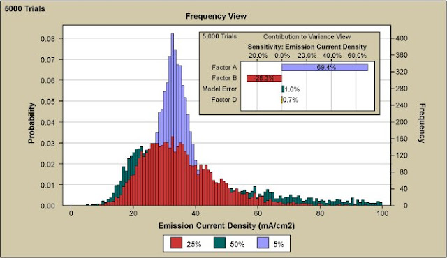
As the variation is increased it can be seen that the curve broadens considerably. However, the broadening disproportionately occurs at the upper end of the emission curve while no important effect is observed at the low end of the spectrum. Only the introduction of a much higher value than the experimental set point in combination with greater variation of Factor B, as seen in Figure 7 allowed for the extension of the emission current histogram towards zero emission and thus achieve a good fit to the measured data. In the figure, Factor B and its variation on emission current density curve came from 5000 simulation trials. Factor A variation was held constant at 50 percent.
Figure 7: Simulation Software Output Showing Influence of Factor B
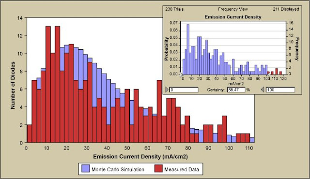
Figure 8: Overlay Plot of Monte Carlo Simulation of Emission Current Density and Measured Data
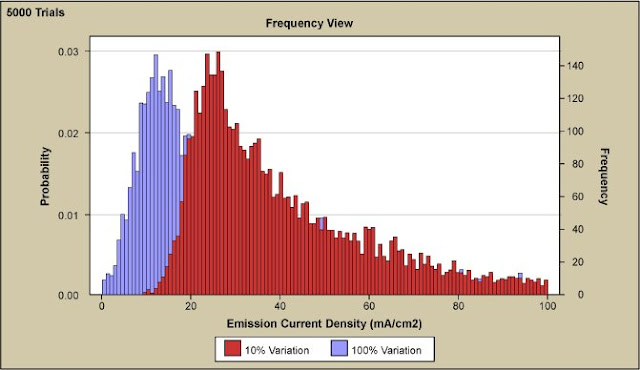
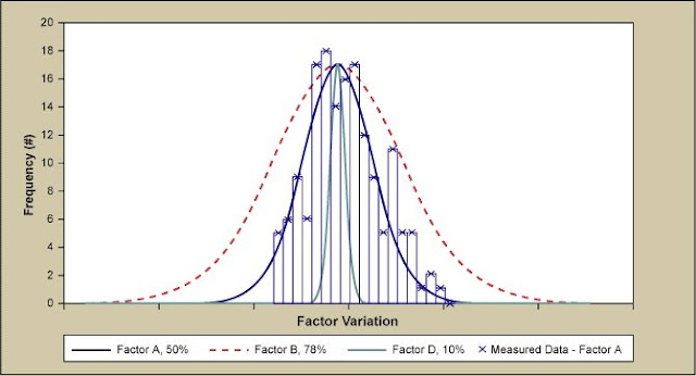
The resulting final fit to the measured emission current density output distribution is shown in Figure 8. The fit was obtained with a 50 percent variation of the most significant Factor A, 78 percent variation of Factor B and Factor D stayed at 10 percent variation. Inset is a simulated run with the same amount of runs as the measured data.
The curve of measured data appear somewhat serrated compared to the fitted curve which may be explained by the limited number of 230 data points when compared to about 4 million simulated data points. The inset of Figure 8 shows the result of a simulation with only 230 runs (i.e., the equivalent number of measured data). The graph is very similar to the measured data, as it displays again a certain degree of unevenness and some bins that are not occupied. Therefore, the discretization of the data seems to be due to the low number of measured data relative to the simulation. As mentioned, during the improvement process the measuring of Factor A run-to-run variation was initiated. As illustrated in Figure 9, the measured Factor A variation has a standard deviation of 42 percent of the mean and agrees quite well with the 50 percent of simulated curve. Also shown are the Factor B and D variation.
Figure 9: Distributions of All Process Input Factors After Good Fit to Measured Data
The high Factor B variation was unexpected. The large fluctuation of Factor B was directly related to an underlying factor that dramatically decreased the emission current density. The morphology was crucially influenced by any fluctuations or drift in Factor B. The instrumentation that controlled Factor B was indicating no drift and the important influencing underlying factor was not known at the time, thus leading to the drift.





0 comments:
Post a Comment