Usage-based Models Improve Odds in Software Testing

The need to test products of all kinds, software and physical products, often runs into challenges connected with:

◉ What to test?

◉ How to test?

◉ How long, how many tests to run?

◉ How to document the risk remaining after test?

Software is particularly challenging because the properties worth exercising and assessing in tests are hard to see and measure, and sometimes even hard to define. While there are no silver bullets, there are some approaches to testing that improve the odds of finding the most important software operational and performance weaknesses with reasonable investments of time and resources. One such test approach, often called usage-based, has statistical roots and some connections that Lean Six Sigma Black Belts could effectively support and perhaps evolve.

Approaches to Software Test

One way to sort out test strategies is by the way each one looks at and plans to exercise the unit, component or system of interest. Such sorts might be:

◉ Internal, Path and Logic View: Looks at software from the perspective of its executable image in a target system. Testing in this view, involves covering the logical pathways through that image (branches, loops, etc.) and tracing the implications of that image on the target system (memory allocation and release, timing, etc.) Classic tools like McCabe’s complexity analysis and an evolving set of new tools are able to inform and focus test planning and analysis from this gutsy inside view of the software in action.

◉ Combinatoric View: Views software and related systems in terms of the combinations of components and infrastructure that may find themselves having to work together. For example, a software product may have to run in combination with various peripherals, browsers, operating systems, network protocols, etc. Testing, from this perspective often involves finding an efficient subset of all possible combinations (which might be overwhelmingly hard or time-consuming to do). The Six Sigma eye for fractional experimental designs sometimes sees this as an opportunity – but not without risk that should be understood.

.

◉ Usage-based Models: Look at a system, at a useful level of granularity, from the perspective of the states, transitions, events and actions that can describe its behavior at that level. As testing may involve simulating events and documenting the actions that ensue, such a model will scope out what complete coverage would look like (the exhaustive array of potential tests) – but, more usefully, it can help identify a statistically efficient subset of those tests that might be worth running first.

A Stochastic Network, or Markov Chain

A states-and-transitions view of any system, where the future behavior only depends on the current state (i.e., it is memory-less) may be modeled as a stochastic network or, more commonly, a Markov Chain (for the mathematician Andrey Markov).

In software, a state machine may often have this property – as the way a state machine will respond to a next event depends only on its current state (not how it got there or what happened prior).

Here is a simple example to walk through the steps involved in building and using a software system Markov Chain. In doing so, some key ways that the model can help inform test planning and assessment can be explored.

Creating and Using a Usage-based Model

1. Understand the scope of users, requirements and system behavior detail to be modeled. Usage-based implies a sense of the scope and nature of actor-triggered events that may be encountered. Sometimes this depends on the class of users (e.g., experts, new users, special-purpose users).

Once clear about what is meant by users, then, which range of requirements and specifications will be in the scope of the model? While it may be tempting to set out to model all aspects of a broad system – common sense and other reality often dictates some divide-and-conquer thinking that carves out parts of the system for test in any one endeavor.

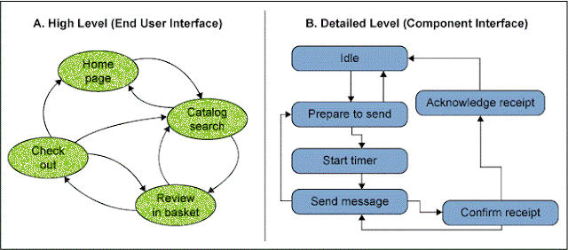
Given the user and requirements scope, the related question to answer is: What level of detail? Is it at the highest level, looking at end-user interface events and actions, or at a finer granularity, looking at components and messages triggering actions in side the system? Figure 1 illustrates the range of granularity that a usage-based approach might span. At the high level, a user with keyboard and mouse are often the interface of interest. Transitions and new states mean things like webpage or screen changes

A lower level may depict the interfaces of objects and components, where transitions involve the messages sent and methods invoked. There is a branch of usage-based test at this component level that makes use of things like Unified Modeling Language (UML) state diagrams to build usage-based views. As a simple introduction, it is best to follow the higher-level view. Once understood, many of the same notions apply in the finer granularity views.

Figure 1: Usage Model Level of Granularity

2. Identify the states and transitions that describe behavior of interest. This is not always as easy as it sounds – but it can actually be an added value part of this approach. The process of thinking through “what are the states and transitions?” may help designers, developers and test people uncover things they were not mutually clear about and to reach a better shared understanding of the system they are working on together. Doing this before design and coding are done is most beneficial, as that shared understanding can prevent defects from being inserted in the first place – the best impact of testing one could hope for.

Figure 1A is a simple view of a high-level states and transitions map. Each state is in a bubble and each transition shown with a directed arc indicating the change from the one state to the other. Note that a state may loop back on itself (e.g., on the home page and clicking home page).

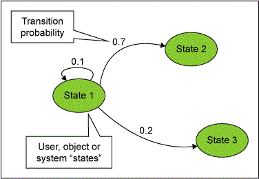
3. Estimate transition probabilities or long-range likelihood. Figure 2 illustrates a simple case with probability (the formal Markov terminology) or long-range frequency (the equivalent-enough practical meaning) labeled on each arc to show how often that transition would be expected to happen. Transitions can be thought of as one of two ways:

◉ Event-triggered: A mouse click or keyboard input, for example. The frequency depicts what proportion of the events will trigger this transition?

◉ Time-slice-triggered: Where the frequency depicts in the next time-slice (e.g., 10 seconds, 1 minute) with what frequency will one expect to find the system in which related state?

In this case, the article will proceed with an event-driven view.

Figure 2: States, Transitions and Probabilities (Long-range Frequencies)

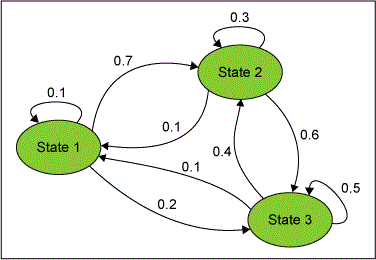
Figure 3: A Completed States and Transitions Diagram

4. Use the Model to Inform Test Case Sampling Plans. Once the states and transitions model is built it can be used in a few ways.

Review of Stationary Distribution

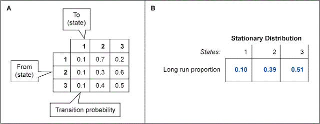
An interesting property of Markov Chains is the review of stationary distribution. In simple terms, this means: “What is the long-range frequency with which we’d expect to see each of the states happening?”

Figure 4A shows a simple Markov Chain depicted as a matrix. Using that form, the statuary distribution can be directly computed (using some matrix algebra). Figure 4B shows the stationary distribution for the simple states and transitions diagram. The interpretation of that is the system will spend about 59 percent of its time in State 2. That might be a first indication of how to allocate some test time and resource. (Obviously, this is more useful in a more complex case than this introductory example.)

Figure 4: Matrix View of States and Transitions/Can Yield Stationary Distribution

Test Case Sequences

While the stationary distribution gives some general guidance, more concrete test planning help can come from the extraction of test case sequences from the usage model. In simple terms that involve:

◉ Identifying a starting state (often a home page or startup screen for usage models at this high level).

◉ Using the transition probabilities to answer the question: “Which transition would we want to test next?” That usually means following untested transitions with high probabilities of being invoked. But in some test regimes, there may be reliability or cost information that is used in concert with the transition probabilities to guide planning for the next test case.

The table to the right illustrates the first few test cases for this simple example. Note that the first case follows path with highest probabilities, then the next case follows untested paths with the next highest probabilities, etc.

Test Cases

Test No.	Usage Sequence
1	1-2-3-Exit
2	1-3-2-Exit
3...	Etc…

5. Assess test results.

What Lean Six Sigma Brings to the Equation

Like a lot of things in the Lean Six Sigma world, the science of usage-based testing originated and evolves outside of Six Sigma – but the practitioner’s toolkit, and potentially that science, can be advanced by bringing the practice onto the Six Sigma radar. Black Belts and project team members can bring their Six Sigma skills to bear in a number of ways that could strengthen usage-based testing, while deriving some benefits as they tailor it to their software test process:

◉ Understanding of the statistics and heuristics involved in Markov Chains and computational intelligence search and sampling methods. Black Belts benefit by understanding stochastic models, and Markov Chains may show up in projects as diverse as software test and Lean systems operations.

◉ Providing guidance in measurement system and sample size. When it comes to the sampling questions about how many test cases to run, and how to measure performance for particular test cases, Black Belts may be quite helpful.

◉ Assessing results. Here is another chance to separate signal from noise using good Six Sigma principles. In some cases, the model may assess costs and reliability-modeled performance in certain states. The Six Sigma infrastructure can help a test organization get a handle on the right mathematical and logical ways to assess raw test results.

◉ Reporting of results in convincing technical and business terms. As it works out in many other aspects of Six Sigma work, sometimes a critical link in the chain of planning and learning that accompany an analysis is the way the implications to the business and technology are understood and reported. Black Belts can help this testing science be better understood by the business and technologists outside of the test talk arena.